Jacob Schwartz Scientist & HTML fan
The wrong (and right) way to select random velocities of particles moving through a surface
Part of my thesis is about simulating gases inside a box: their flow and how they interact with a plasma that is also inside a box. In order to do this, I’m using a FORTRAN code that’s been developed by generations of graduate students. I ran a simple test case in which I should end up with a gas of a uniform temperature and density inside my box, but to my horror the temperature was lower than expected. In my test case, I model the box boundaries as surfaces beyond which is a resevoir of a stationary gas in thermal equilibrium. The code works by launching particles from the boundaries, as if they had come from that reservoir, and tracking their passage through the box. For this test, there are no collisions between the particles; they were turned off. I realized there was a problem how particles are assigned an initial velocity, starting from the boundary. It was a conceptual error about the correct probability distribution from which to draw the velocities.
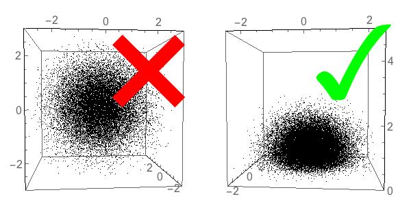
How NOT to launch particles from the wall.
A stationary gas in thermal equilibrium is isotropic: particles have an equal chance of moving in all directions. Let’s normalize the velocities to a standard thermal velocity, $v_{th} = \sqrt{T /m}$. In Figure 1, points represent the velocity vector of such particles. Each of $v_x$, $v_y$, and $v_z$ are drawn from a Gaussian distribution with a mean $\mu=0$ and standard deviation $\sigma = 1$.
\[\begin{equation} f(v_x, v_y, v_z) = \frac{1}{\left(2 \pi \right)^{3/2}} \exp\left(-\frac{v_x^2 + v_y^2 + v_z^2}{2}\right) \tag{1}\label{eq:max} \end{equation}\]The mean of the square of any velocity component is 1, and since they are independent, the mean of the full $v^2$ is 3:
\[\begin{equation} \left< v_x^2 \right> = \left< v_y^2 \right> = \left< v_z^2 \right> = 1, \qquad \left<v^2\right> = \left< v_x^2 \right> + \left< v_y^2 \right> + \left< v_z^2 \right> = 3 \tag{2}\label{eq:maxv} \end{equation}\]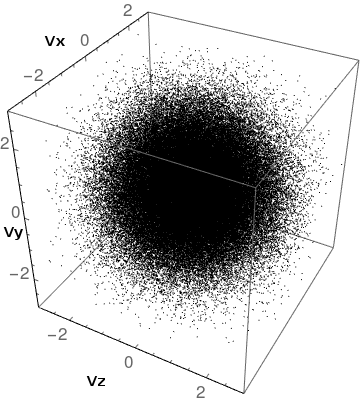
The fundamental conceptual problem
If we were modeling a volumetric source of particles (perhaps if were starting another type of simulation with particles already inside a box), this would be the correct distribution from which to draw. However, we are modeling particles that have crossed an imaginary planar boundary from the outside (stationary Maxwellian) reservoir into our simulation space. The fact that these particles had to cross the planar boundary means that their velocity through that boundary must be positive. Additionally, particles with faster speeds normal to the boundary are more likely to cross that boundary.
As an example of the last statement, imagine cars in two lanes on a highway: one lane with cars moving at 1m/s, and the other with cars moving at 100m/s. Assume that the cars in both lanes are spaced 100 m apart. A person standing on the side of the road will see one fast car pass per second, and one slow car only once per 100 seconds. Yet, the density of cars per kilometer in each lane is the same.
The fix
We need to include a factor proportional to the speed normal to the boundary. Let the direction normal to the boundary be $\hat{z}$, so the extra velocity factor is $v_z$. The velocity distribution of particles crossing the boundary is
\(\begin{equation} g(v_x, v_y, v_z) = \frac{1}{2 \pi } v_z \exp\left(-\frac{v_x^2 + v_y^2 + v_z^2}{2}\right). \tag{3}\label{eq:maxray} \end{equation}\) This is the distribution we need to draw from when launching particles from the simulation boundary.
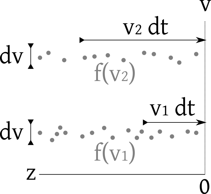
Figure 2 illustrates why the factor of $v_z$ is necessary. Particles moving with $\hat{z}\text{-velocity}$ $v_z$ can make it across the boundary in time $dt$ if they are at a distance $v_z\;dt$ or less from the boundary. The density of particles in a given velocity increment $dv_z$ is proportional to $f(v_z)$, so the number of particles in that increment that cross a boundary in a time $dt$ is equal to $f(v_z) dv_z \; v_z \; dt$. Note that while $f(v_1) > f(v_2)$ for $v_1 < v_2$, it is possible that $v_2 f(v_2) > v_1 f(v_1)$, as shown in the figure.
The particles from the distribution in Equation 3 have $v_x$ and $v_y$ distributions identical to those from Equation (1), but the $v_z$ distribution is changed to what is termed a Rayleigh distribution.
It is constrasted with a half-Gaussian distribution in Figure 3, below. There are two notable features: first, the value of the distribution tends to zero as $v_z \to 0$; particles moving very slowly don’t cross your boundary of choice very often. Second, the probability-mass is skewed to the right compared with the half-Gaussian; fast-moving particles cross boundaries more often.
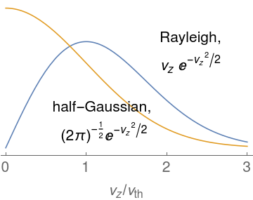
The Rayleigh distribution has the property that $\left<v_z^2\right> = 2$, thus, $\left<v^2\right> = 4$, so (dropping the $v_{th} = 1$ normalization for a moment) the average energy $\left<\frac{1}{2} m v^2\right>$ of particles moving through a surface is $2 T$, not the $\frac{3}{2} T$ of particles in a volume of equilibrium gas. In the original, flawed code, the injection of particles with the lower average energy associated with a half-Gaussian led to the anomalously low temperature I saw.
Incidentally, the Rayleigh distribution is also is identical to the distribution of radial velocity $v_r = \sqrt{v_x^2 + v_y^2}$.
Sampling from the Maxwellian-influx distribution $g$.
Sampling $g$ requires drawing three random numbers1 rand $\in (0, 1]$: one each for the radial and z velocities and one for the angle. Sampling from the $f$ distribution is similar2.
vr = SQRT(-2 * LOG(rand))
theta = 2 * PI * rand
vx = vr * COS(theta)
vy = vr * SIN(theta)

vz = SQRT(-2 * LOG(rand))
It works!
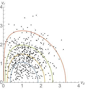
I ran this algorithm and checked that the velocities had the correct properties. I also had some fun visualizing the level curves of the distribution $g$.
Even better, I was able to add the algorithm to the code and saw that it fixed my launched particles!
Bonus: drawing the contour lines.
Let’s recast $g(v_x, v_y, v_z)$ into $G(v_r, v_z)$:
\[\begin{equation} G(v_r, v_z) = \frac{1}{2\pi} \exp(-v_r^2/2)\,v_z \exp(-v_z^2/2) \end{equation}\]Solve for $v_r$ as a function of $v_z$ such that $G$ equals some contour value $h$:
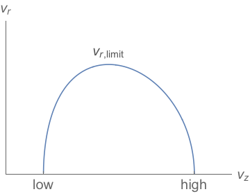
\[\begin{equation} v_{r,\text{limit}} = \sqrt{2 \log\left(\frac{v_z}{2 \pi h}\right) - v_z^2} \end{equation}\]This expression equals zero at two points. I used Mathematica to find those low and high limits,
\[\begin{equation} \text{low} = 2 \pi h\,e^{-\frac{1}{2} W_0(-4 \pi^2 h^2)}, \quad \text{high} = 2 \pi h \, e^{-\frac{1}{2}W_{-1} (-4 \pi^2 h^2)}, \end{equation}\]where $W$ is the Lambert W function, defined such $W(z)$ gives the solution for w in $z = w \exp(w) $. As a clarification, the meaning of these points is shown in Figure 5:
We need to find the amount of $G$ inside this contour for a given $h$. Integrate $G$ in the $v_r$ and $v_z$ directions:
\[\begin{align} \int_{\text{low}}^\text{high} v_z \int_0^{v_{r,\text{limit}}} v_r\,dv_r \, 2 \pi\,G &= 4 \pi ^2 h^2 e^{-\frac{1}{2} W_0\left(-4 \pi ^2 h^2\right)}-4 \pi ^2 h^2 e^{-\frac{1}{2} W_{-1}\left(-4 \pi ^2 h^2\right)} \\ &+ e^{\frac{1}{2} W_0\left(-4 \pi ^2 h^2\right)}-e^{\frac{1}{2} W_{-1}\left(-4 \pi ^2 h^2\right)} \tag{4}\label{eq:contourlevel} \end{align}\]To find the contour level $h$ such that a fraction $a$ of samples lie inside that contour, set Equation (4) equal to $a$ and use a root finder.
Mathematica:
getLevelH[a_] :=
 h /. FindRoot[
   E^(1/2 ProductLog[-4 h^2 Pi^2]) - E^(
     1/2 ProductLog[-1, -4 h^2 Pi^2]) +
     4 E^(-(1/2) ProductLog[-4 h^2 Pi^2]) h^2 Pi^2 -
     4 E^(-(1/2) ProductLog[-1, -4 h^2 Pi^2]) h^2 Pi^2 ==
    a, {h, 10^-10, 1/(2 Pi) Exp[-1/2]}]
-
If your RNG supplies values $\in [0, 1)$ it could be wise to use the value’s complement with one to avoid
LOG(0). ↩ -
A simple method to sample from the Maxwellian (3D Gaussian) distribution $f$:
vr = SQRT(-2 * LOG(rand))
theta = 2 * PI * rand
vx = vr * COS(theta)
vy = vr * SIN(theta)

t0 = SQRT(-2 * LOG(rand))
t1 = 2 * PI * rand
vz = t0 * COS(t1)
This certainly isn’t the best algorithm since it requries four random samples for only three velocity dimensions. ↩