Radial profiles of deposition in a disk: a tricky Taylor series

The previous post calculated the fraction of particles encountering a 2D disk which pass though the disk before being absorbed (deposited) with some mean free path $\lambda$. This post calculates the radial profile of the intensity of deposition in the disk: the number of particles are deposited per unit area at radius $0 \lt \rho \lt 1.$

A disk of radius $1$ is surrounded by a uniform 2D-isotropic gas of particles. This problem is indifferent to their distribution of speeds; which could be Maxwellian (as a typical gas), or identical (as like photons); interactions depend only the distance travelled through the disk.

Problem background and setup

Background gas

Assume the background density of particles is $1$ per unit length squared and all particles move at a speed of $1$ unit length per unit time. The one-way flux across a unit-length line segment is $\left(\int_{-\pi/2}^{\pi/2} 1 * 1 * \cos\phi\;d\phi\right)/ \left(\int_{-\pi}^{\pi}\;d\phi\right) = 1/\pi$ per unit time, where $\phi$ is the direction of particle motion. Since the disk has circumference of $2\pi$ the rate of particles entering the disk is $2$ per unit time.

Setup for integration

I want to find the intensity of deposition at a given radius $\rho$. This is the total deposition per unit time in the annulus of radius $\rho$ and width $d\rho$ summed over all central angles $\theta$, divided by the annulus area of $2\pi\rho\,d\rho$.

The deposition intensity is

where $y(\phi, \theta, \rho, \lambda)$ is the deposition intensity from particles moving at angle $\phi$, at radius $\rho$ and central angle $\theta$. The $\cancelcolor{\rho}$ in the numerator is the standard Jacobian of polar coordinates. This will cancel with the $\cancelcolor{\rho}$ in the denominator; the $d\rho$s also cancel.

By symmetry, the radial intensity from all angles $\phi$ is the same; thus we can consider an equivalent scenario where all particles come from the same direction, but with $2\pi$ times the intensity. The cover illustration shows all particles entering from the right, with $\phi=\pi$.

For particles coming from a fixed $\phi$, the deposition at the point given by $(\rho, \theta)$ is proportional to $\frac{1}{\lambda}\exp(-d_\mathrm{decay}/\lambda)$, where

The leading $1/\lambda$ is the intensity of deposition from particles with mean free path $\lambda$.

Cancelling the $\cancelcolor{\rho}$, the intensity of deposition at a given radius $\rho$ is

For brevity I will define

so Equation \eqref{eq:one} can be expressed as

The solution as a Taylor series

Unfortunately, we cannot evaluate the integral in terms of elementary functions, or as far as I can tell, even in terms of complicated non-elementary functions like the Meijer-G function.

Instead, I found a Taylor series for $i$ around $\rho=0$. I did this by expanding $f$ in a Taylor series and integrating each term.

The deposition intensity $i(\rho,\lambda)$ is

The shape of ${i}$

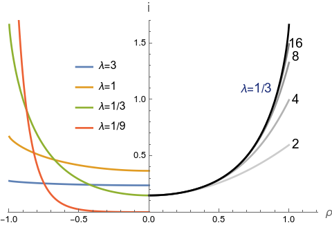
The left half of Figure 3 shows plots of ${i}(\rho, \lambda)$ at various $\lambda$ and the right half shows the accuracy of Taylor series out to various orders.

Special cases: center and edge

For $\rho=0$ and $\rho=1$ the expression for $i$ can be directly integrated. The deposition intensity at the disk center is $i(\rho=0, \lambda) = \frac{1}{\lambda}\exp(-1/\lambda)$, which has a maximum of $e^{-1}$ at $\lambda=1$.

The deposition intensity at the disk edge is

where $_0\tilde{F}_1$ is the regularized hypergeometric function and $\pmb{L}_0$ is the ever-popular modified Struve function.

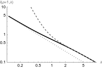
At small $\lambda$,

and at longer $\lambda$ it goes like

Numerical check of the solution

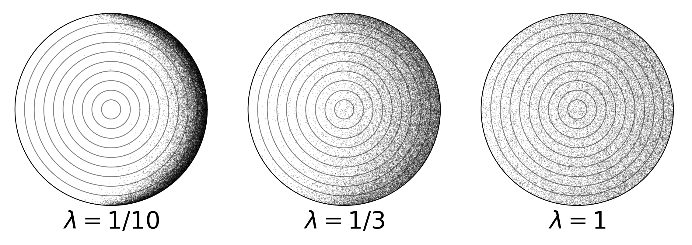
As a check I wrote a numerical simulation of particles (coming all from one angle). Figure 4 visualizes the deposition locations for different $\lambda$.

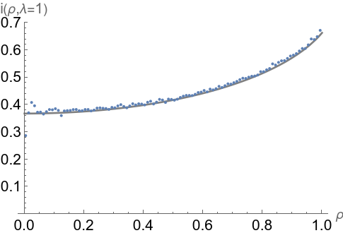
In Figure 5 is a histogram of the radii of 2 million points with $\lambda=1$. There is significant scatter near the origin, even with so many particles, demonstrating the value of the analytical solution.

The rest of the post will derive the Taylor series expression for $i$. As a word of caution it is complex. Only read on if you really want to.

0. Outline of the derivation

Equation \eqref{eq:two}, repeated here, is

where $ f \equiv \exp\left(-\left(\sqrt{1 - \rho^2 \sin^2\theta} - \rho \cos\theta\right)/\lambda\right)$.

I will express $f$ as a Taylor series:

where $j_n(\lambda, \theta)$ are functions of $\theta$ and $\lambda$. By the standard Taylor series construction,

Then

I reverse the order of the sum and integral (and move left the $\rho^n/n!$) to get a Taylor series for $i$,

where I’m defining

I will show that each $j_n(\lambda, \theta)$ is a sum of terms of the form

where $w$, $s$, $b$, and $g$ are non-negative integers, and further, $b$ is even.

Then, $l_n$ is a polynomial in $1/\lambda$,

where $u_{n,k}$ are ratios of integers. The coefficients $w$ and then $u_{n,k}$ will be found by carefully analyzing the derivative-taking process. It will turn out that $u_{n,k}$ is best expressed as a sum over a third index, which I’ll call $c$.

1. The derivative-taking game

Taking repeated derivatives of $f$ with respect to $\rho$ yields sums of terms of the form

where $w$, $r$, $s$, $b$, and $g$ are non-negative integers, and $m$ can be an integer or half-integer $(0, 1/2, 1, 3/2, \ldots)$.

For example the first derivative is

and the second derivative is

Examining the derivative process more closely, let’s take the derivative with respect to $\rho$ of a general one of the Expression $\eqref{eq:rsqform}$-type terms. The existing $w \sin^{2s}\cos^b/\lambda^g$ are independent of $\rho$, so I will ignore them.

Thinking of a term with some combination of ${r, m, s, b, g}$ as a point in a 5-d space, the derivative operation on a point with initial weight $w=1$ yields up to four new points with associated weights $1$, $1$, $2m$, and $r$:

The four derivative steps:
    {r+1, m+1/2, s+1, b  , g+1}   # A
+   {r  , m    , s  , b+1, g+1}   # B
+ 2m{r+1, m+1  , s+1, b  , g }    # C
+  r{r-1, m    , s  , b  , g }    # D

# These are in the same order as the terms in Eq (6).

I say up to four new points because if $m=0$ (as in the base $f$) or if $r=0$ (also in the base $f$, and along paths where $r$ increased and then decreased to zero) then those terms will not be generated. I’ve labeled the four new points, or steps, as $A, B, C, D$.

Here’s a diagram that shows this in action:

Using a computer algebra system like Mathematica, it’s not difficult to take derivatives, then set $\rho$ to 0, then integrate over $\theta$ to find the polynomial $l_n(\lambda)$.¹ But, it would be still be interesting to come up with a closed-form expression for $l_n(\lambda)$.

2. The pattern of derivatives

In order to get closer to a closed-form expression for $l_n(\lambda)$, let’s make some observations about the patterns of derivatives, or the patterns of steps, as in the diagram.

2.1 Only r=0 terms survive in $j_n$

The $n’th$ derivative is the sum of all permutations of length $n$ of ${A,B,C,D}$.

After taking the derivatives, the next step in forming $j_n$ is to set $\rho \to 0$. Only terms with the exponent $r=0$ (in $\rho^r$) will survive. The root term $1$ has $r=0$; steps $A$ and $C$ both increment $r$ and step $D$ decremenets it. Therefore, any surviving term will have

where $a$ is the number of steps $A$, and so on.

2.1 Only even-$n$ $l_n(\lambda)$ are nonzero.

Step $B$ contributes a factor $\cos\theta$ to the numerator. When this is integrated from $0$ to $2\pi$, terms with odd powers of cosine will be cancelled out; only terms with even $b$ will survive. As shown above, surviving terms have $a + c = d$, so $a + c + d$ is even. If $n$ is odd, $(a + c +d) + b$ must be odd as well, so $b$ will be odd. Conversely, if $n$ is even $b$ will be even.

Therefore $l_n(\lambda)$ will be zero for all odd $n$. This means the Taylor series of $i$ only has even powers of $\rho$!

Also, all the terms contributing to even $l_n$ will have $\sin^{2s}\cos^{b}$ with even $b$.

2.2 Restrictions on valid $c$ for given $n, k$

The polynomial $l_n(\lambda)$ is a sum of terms with different powers of $1/\lambda^{n-k}$. For a given $n$ and $k$ there are restrictions on $c$, the number of steps $C$ which can be taken to contribute to a term with $1/\lambda^{n-k}$.

For example, by inspection of the table of steps above, only $A$ and $B$ increase $g$, that is, contribute a power of $1/\lambda$. Thus,

Using Equations \eqref{eq:nabcd}, \eqref{eq:acd}, and \eqref{eq:nkab}, together with the inequalities

we find that for a given $(n,k)$,

From the equations listed above we can express $a$, $b$, and $d$ in terms of $n$, $k$, and $c$:

3. Weights of paths to get to a term

3.1 Factor from the order of (A|C)’s vs D’s

From Equation \eqref{eq:acd}, $a + c = d$. The order of the $A$s, $C$s, and $D$s contributes an extra weight to path because of the coefficient $r$ whenever step $D$ is taken. For example, $AAADDD$ has a weight of $3∗2∗1=6$ but $ADADAD$ has a weight of $1∗1∗1=1$.

As mentioned before, not all paths are valid: all the prefix substrings must have the number of ($A$’s or $C$’s) greater than or equal to the number of $D$’s, or else the weight will crash down to zero (from differentiating a constant).

For paths of length n=4

AADD : weight of 2
ADAD : weight of 1
ADDA : weight of 0
DAAD : weight of 0
DADA : weight of 0
DDAA : weight of 0

I found experimentally² that the sum of the weights of all these paths matches OEIS A001147, which is

where !! is the double factorial.

3.2 Factor from order of A’s and C’s

In the above process, the order of $A$s and $C$s does not matter. But, there is also a weight for each path from the coefficients $2m$, which depends only on the order of the $A$s and $C$s. Each $A$ increases $m$ by $1/2$ and each $C$ multiplies the weight by $2m$ and increments $m$ by $1$.

I simulated³ this process and found that the pattern of the sum of the weights over all permutations of $A$ and $C$ here was basically the same as the Bessel numbers, but with the indices shifted. This yields a factor of

where $(k-2c)_{2c}$ is a Pochhammer symbol. The latter form is preferred over the ratio of two Gamma functions to avoid an intederminate expression when $k=c=0$.

3.3 Factor from insertion of B’s

The steps $B$ can be inserted anywhere in the above sequences without changing the outcome of the $r$-weights or $m$-weights. Thus the number of paths is multiplied by

where $\binom{x}{y}$ is a binomial.

3.4 Harmonic factors

Steps $A$ and $C$ contribute factors of $\sin^2\theta$ while step $B$ contributes $\cos\theta$.

Thus the harmonic part will be

4. Putting the pieces in place for $j$, $l$, and $i$

Setting $\rho$ to zero

When setting $\rho$ to 0 each term like that in Equation \eqref{eq:rsqform} becomes

Construct j

Therefore

Integrate to get $l_n(\lambda)$

For even $b$,

Here $s = a + c = k-c$ and $b=n-2k+2c$. Therefore

and

I’ve moved the $\gfour{2/(n/2)!}$ out to the front because it does not depend on $k$ or $c$.

The first few $l_n$ are

For completeness,

Finally ${i}$

Repeating the relation between $l_n$ and $i$,

we can finally construct $i$:

Putting $l_n(\lambda)$ back into the formula for ${i}$ I was able to combine the $\lambda$ with the others in the denominator and cancel a $2$.

Postscript

Thanks to C. Swanson and J. Parisi for your proofreading, comments, and encouragement.