Sauter shape studies, Part 1: Overview, volume, and cross-sectional area

I’ve been developing a new “systems code” for studying the design and economics of fusion reactors. Fusion reactor systems codes used simplified representations of the various parts of the machine—the plasma, magnets, breeding blankets, electrical generatros, and so forth—in order to be able to compute and reason about aspects of the system as a whole. In this post, I discuss a simple parameterization for the shape of the plasma boundary.

In a 2016 paper, O. Sauter describes a parameterized shape for a plasma boundary,

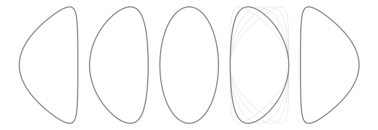
\[\begin{align} R(t) &= R_0 + a \cos\left(t + \delta \sin(t) - \xi \sin(2t)\right) \\ Z(t) &= \kappa a \sin(t + \xi \sin(2 t)), \end{align}\]

where $R_0$ is the major radius, $a$ is the minor radius, $\kappa$ is the elongation, $\delta$ is the parameter for triangularity, and $\xi$ is a parameter for squareness. The title image shows shapes with $\kappa=2, \xi=0$, and $\delta$ of $-0.8$ to $0.8$. Sauter’s motivation is to provide simple formulas for plasma properties that work when $\delta \lt 0$, because negative-triangularity tokamaks have recently been experiencing a resurgence of interest.

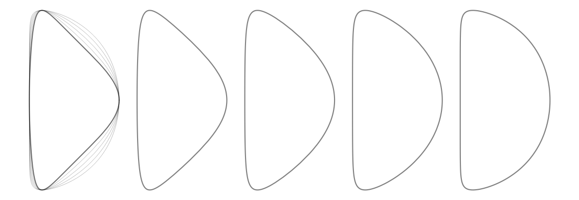
The formulas that he provides also include $\xi$, for ‘squareness’. The effects of varying $\xi$ are shown in Figure 1. For this series of blog posts I’ll generally set $\xi=0$, because otherwise the formulas are too difficult to work with analytically; numerical integration is required for everything.

Figure 1: Sauter plasma boundary shape with $\kappa=2$, $\delta=0.8$, and $\xi$ of -0.1 to 0.1. The leftmost image has the others superimposed.

Sauter provides formulas for geometric properties of a tokamak plasma that has this boundary shape: the poloidal length $L_p,$ the cross-sectional area $S_\phi,$ the surface area $A_p,$ and enclosed volume $V$. He also gives estimates of physical properties: the safety factor $q_{95},$ the plasma current $I_p,$ the average poloidal magnetic field along the last closed flux surface $B_p,$ and the fraction of trapped particles $f_t$. At the moment I’m more concerned with the geometric properties, but I plan to address $f_t$ later.

Remarks on the shape and other models

The formulas $R(t), Z(t)$ are heuristic approximations and not based on physical principles: they break in unphysical ways (self-intersection or cusps) when $\delta$ or $\xi$ are too large.

A first approximation to a tokamak plasma shape is often an ellipse. This corresponds to Sauter’s formulas with $\delta= \xi=0$.

For a more general model, Jean Johner’s HELIOS code uses a last closed flux surface (LCFS) shape made of four conic section arcs. This permits plasma with different upper and lower $\kappa$ and upper and lower $\delta$, and also sharp angles for one or two X-points. One drawback is the greater number of cases (ellipse, parabola, hyperbola) which must be implemented.

Basic geometry of the triangular Sauter shape

Let’s set $\xi=0$ and normalize the equations by dividing by $a$:

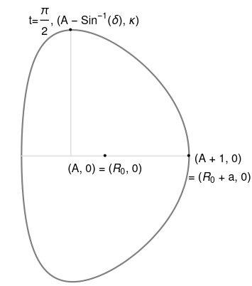
\[\begin{align} R_A(t) &= A + \cos\left(t + \delta \sin(t)\right) \\ Z_A(t) &= \kappa \sin(t), \end{align}\]

where $A \equiv R_0 / a$. I’ll later use $\epsilon \equiv a / R_0 = A^{-1}$.

The LCFS always has maximum height $\kappa$. The ‘crown’ is at $R_A(t = \pi/2) = A - \sin^{-1}(\delta)$.

Figure 2: Points of interest on the (normalized) triangular Sauter shape.

Sauter calls the curve parameter $\theta$ whereas I call it $t$; I found the former confusing because $\theta$ is not the angle between the plasma axis and a point on a curve. That angle is given by $\theta_c(t) = \tan^{-1}(R_A(t) - A, Z_A(t))$.

Non-parametric forms

We cannot solve for Z(R). However, we can find $R_A(Z_A)$:

\[R_A - A = \pm \cos\left(\frac{Z_A \delta}{\kappa} \pm \sin^{-1}\left(\frac{Z_A}{\kappa}\right)\right)\]

I do not think there a convenient polar form, for distance to the LCFS parameterized by the angle around the plasma axis $\theta_c$.

Exact results and derivation of approximations

Sauter presents approximate formulas for $L_p,$ $A_p,$ $S_\phi,$ and $V$. As far as I can tell, these are based on numerical fits to collections of plasmas with various shapes, including $\xi \ne 0$ and plasmas which are not up-down symmetric. Since I’m less interested in $\xi$, it would be nice to have a collection of formulas specifically for $\xi = 0$. And for self-consistency’s sake it would be good to have close matches to use with exact moments from numerical integrations that I might need to do later.

Poloidal cross-section area

Rather than a double integral in Cartesian coordinates $\;dR \; dZ$ it’s convenient to integrate directly from the parametric form $R(t), Z(t)$. The poloidal cross-section area is

\[\begin{align} S_\phi &= \int_0^{2\pi} -Z(t) \frac{d R}{d t} \; dt = 2 a^2 \int_0^\pi - Z_A(t) \frac{d R_A(t)}{d t}\;dt \\ &= 2 a^2 \kappa \int_0^\pi (1 + \delta \cos t )\sin(t + \delta \sin t )\sin t \; dt. \end{align}\]

The integral evaluates to $\pi J_1(\delta) / \delta = (\pi/2)\left(J_0(\delta) + J_2(\delta)\right)$, with the second form preferred to avoid dividing by zero. The cross-section area is

\[S_\phi = \pi a^2 \kappa (J_0(\delta) + J_2(\delta)).\]

This form is nice because the leading terms are the area of an ellipse; the Bessel functions act as a correction factor of order 1 for the triangularity. This is shown in Figure 3.

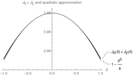
Figure 3: Correction factor to the poloidal cross-section area for triangularity. The quadratic approximation is shown in lighter gray.

If you don’t want to use a Bessel function, the correction factor can be approximated by $\left(1 + \delta^2/8 + \delta^4/192\right)$. With the quadratic term only it’s good to within a factor of 1.006 when $-1 \lt \delta \lt 1$ and with the quartic term it’s good to within a factor of 1.00012.

This exposes the first tiny ‘rift’ between my formulas and Sauter’s. His formula uses a correction factor of $(1 - 0.1274 \delta^2)$ whereas mine is $(1 - 0.125 \delta^2)$. Gasp!

Volume

The enclosed volume of the plasma is

\[\begin{align} V &= \int_0^{2 \pi} - Z(t) 2 \pi R(t) \frac{d R(t)}{d t} \; dt \\ \frac{V}{2 \pi^2 R_0 a^2 \kappa} &= \frac{2}{\pi} \int_0^\pi (1 + \delta \cos t )\left(1 + \epsilon \cos(t + \delta \sin t )\right) \sin(t) \sin(t + \delta \sin t )\;dt \end{align}\]

The second line is formulated so that the right hand side is a correction to the volume of an elliptical torus. The right hand side evaluates to $J_0(\delta) + J_2(\delta) - (\epsilon/4) (J_1(2 \delta) + J_3(2 \delta))$. The first two functions are the ones we encountered above, and the $J_{\nu=\mathrm{odd}}$ functions are odd functions of $\delta$. This correction factor can be approximated using the four-term series

\[1-\frac{\delta ^2}{8}-\frac{\delta \epsilon }{4}+\frac{\delta ^3 \epsilon }{12}\]

which is correct to within a factor of 1.012 for $-1 \lt \delta \lt 1$ even when $\epsilon = 2/3$, a very low aspect ratio. Sauter’s formula, which has different numerical coefficients for the same powers, is only good to within 5% over this range. For a bit more accuracy

\[1-\frac{\delta ^2}{8}+\frac{\delta ^4}{192}-\frac{\delta \epsilon }{4}+\frac{\delta ^3 \epsilon}{12}-\frac{\delta ^5 \epsilon }{96}\]

is accurate to within a factor of 1.0006.

Poloidal length and surface area.

These are a bit trickier so I will leave them to Part II!

Written on April 10th, 2021