Sauter shape studies, Part 2: poloidal circumference and surface area

This post is a continuation of the previous, so read that one first. In this post I’ll describe my efforts to compute an approximation for the poloidal circumference and surface area for Sauter’s shape, in the special case of $\xi=0$.

In a 2016 paper, O. Sauter describes a parameterized shape for a plasma boundary,

\[\begin{align} R(t) &= R_0 + a \cos\left(t + \delta \sin(t) - \xi \sin(2t)\right) \\ Z(t) &= \kappa a \sin(t + \xi \sin(2 t)), \end{align}\]

If we set $\xi=0$, we can can put this in terms of $R_A(Z_A)$:

\(R_A - A = \pm \cos\left(\frac{Z_A \delta}{\kappa} \pm \sin^{-1}\left(\frac{Z_A}{\kappa}\right)\right)\).

These are coordinates where we’ve normalized out $a$ and $A$ is the aspect ratio.

Poloidal circumference

Poloidal circumference only depends on the shape of the LCFS and not the aspect ratio, so we can drop the $A$ term from the LHS. We’ll label the two branches of the $\pm$ as $R_i$ for the inner $(-)$ and $R_o$ for the outer ($+$). Thus

\[\begin{align} R_i &= -\cos\left(\frac{z \,\delta}{\kappa} - \sin^{-1}\left(\frac{z}{\kappa}\right)\right) \\ R_o &= +\cos\left(\frac{z\, \delta}{\kappa} + \sin^{-1}\left(\frac{z}{\kappa}\right)\right), \end{align}\]

where for convenience I’m now writing $Z_A$ as $z$.

The exact poloidal length is

\[\begin{equation} L_{p,\mathrm{exact}} = \int_{-\kappa}^{\kappa} \sqrt{1 + R_i'^2} + \sqrt{1 + R_o'^2} \; dz \quad (1) \end{equation}\]

where $R’$ is the derivative with respect to $z$. Unfortunately this cannot be integrated exactly, even in terms of special functions.

Sauter’s expression for the poloidal circumference is

\[\begin{equation} L_{p,\mathrm{Sauter}} = 2 \pi ( 1 + 0.55 (\kappa-1))(1 + 0.08 \delta^2)(1 - 0.049 \delta^2). \end{equation}\]

This is first order in $\kappa$ and fourth order in $\delta$.

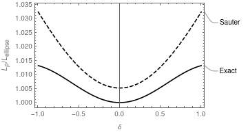
Figure 1 shows the exact formula and Sauter’s approximation. Notice that the latter, despite being 4th order in $\delta$, doesn’t have the downward bends at high $\delta$ like the exact formula does, and that it’s off by about 1% for $\delta=0$. We’ll see if we can derive a more accurate expression with the same powers of $\kappa$ and $\delta$.

Poloidal circumference: Exact in elongation, fourth order in triangularity

Our first step is to expand the integrand of the exact formula as powers of $\delta$. To 2nd order,

\[\begin{align} &\sqrt{1 + R_i'^2} + \sqrt{1 + R_o'^2} =\\ &\frac{2}{\kappa} \sqrt{\frac{\kappa ^4-z^2 \left(-1+\kappa ^2\right)}{-z^2+\kappa ^2}}+ \frac{\left(6 z^2 \kappa ^6+z^4 \kappa ^2 \left(2-13 \kappa ^2\right)+z^6 \left(-3+7 \kappa ^2\right)\right)}{\kappa ^3 \sqrt{-z^2+\kappa ^2} \left(\kappa ^4-z^2 \left(-1+\kappa ^2\right)\right)^{3/2}}\delta^2. \end{align}\]

When integrated from $-\kappa$ to $\kappa$ as in Equation (1) this becomes \(4 \kappa E\left(1-\frac{1}{\kappa ^2}\right) + \frac{2 \kappa \left(2 \kappa ^2 \left(11+5 \kappa ^2\right) E\left(1-\frac{1}{\kappa ^2}\right)-\left(9+20 \kappa ^2+3 \kappa ^4\right) K\left(1-\frac{1}{\kappa ^2}\right)\right)}{3 \left(-1+\kappa ^2\right)^3}\delta^2. \quad (2)\)

Note that the first term is just the formula for the circumference of an ellipse, so the second term is the first correction for triangularity. Taking the Taylor series to the power $\delta^4$ adds to Equation (2) the term

\[\begin{align} & \frac{\delta^4}{90 (\kappa^2 - 1)^6} \\ & \left(-\kappa ^3 \left(3145+27028 \kappa ^2+25854 \kappa ^4+5156 \kappa ^6+257 \kappa ^8\right) E\left(1-\frac{1}{\kappa ^2}\right)\right. \\ & \left.+4 \kappa \left(225+3515 \kappa ^2+7446 \kappa ^4+3630 \kappa ^6+529 \kappa ^8+15 \kappa ^{10}\right) K\left(1-\frac{1}{\kappa ^2}\right)\right) \quad (3) \end{align}\]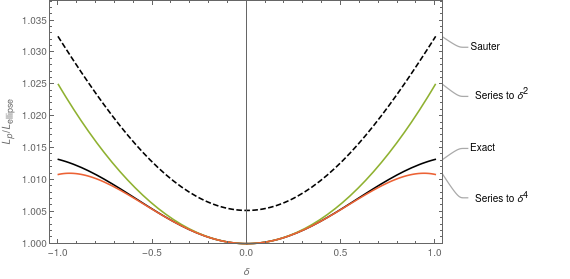

Figure 2 shows these two approximations in $\delta$. They are exactly correct when $\delta=0$ and with the addition of the $\delta^4$ term the flattening near $\delta=1$ is captured.

This might already be a decent place to stop. Though the formula up to 4th order is somewhat complicated, it works well, and only requires one evaluation each of the elliptic integrals $E$ and $K$.

Relieving ourselves of special functions

But what if we don’t like special functions? Can we construct a decent approximation without using them? YES.

First, we use Ramanujan’s ellipse perimeter formula to replace the $\delta^0$ term: \(4 \kappa E\left(1-\frac{1}{\kappa ^2}\right) \approx \pi \left(3(\kappa+1) - \sqrt{(3 + \kappa)(1 + 3 \kappa)}\right)\). This is a very good approximation and will ensure that the formula is correct to about 1 part in $10^5$ when $\delta=0$. That leaves the $\delta^2$ and $\delta^4$ terms. I choose to expand each of these to first order in $\kappa$, centered around a typical elongation of $\kappa=1.5$. The result is

\[\begin{align} L_{p,\mathrm{custom}} &= \pi \left(3(\kappa+1) - \sqrt{(3 + \kappa)(1 + 3 \kappa)}\right) + \\ & \left(0.32131 - 0.162809 (\kappa-1.5)\right)\delta^2 + \\ & \left(-0.157018 + 0.0350393 (\kappa -1.5)\right)\delta^4. \quad (4) \end{align}\]

For reasonable values of $\kappa$ this custom series is within about 0.2% of the series given by Equations (2) and (3).

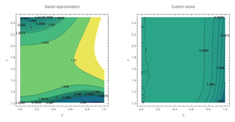
Figure 4 shows a comparison of the Sauter approximation to the ‘custom’ series of Equation (4). I feel satisfied with this level of accuracy.

Poloidal surface area

In this section I’ll derive an approximation for the surface area using elementary functions.

I use the same technique as above: write down the integral for surface area, expand the integrand in powers of $\delta$, integrate each term, and than expand each term in a power of $\kappa$.

The expression for surface area (normalized by $a^2$) is

\[\begin{equation} A_p = 2 \pi \int_{-\kappa}^{\kappa} (A + R_i)\sqrt{1 + R_i'^2} + (A + R_o)\sqrt{1 + R_o'^2}\; dz. \end{equation}\]

Expanding the integrand to zeroth order in $\delta$ and integrating yields the expression for the surface area of an elliptic torus, $8 \pi A \kappa E(1 - 1/\kappa^2)$. Each higher order term contains one instance each of $E$ and $K$ multiplied by polynomials of $\kappa$. For example, the $\delta^1$ term is

\(\delta \int_{-\kappa }^{\kappa } -\frac{4 \pi z^2 \left(-2 \kappa \sqrt{\frac{-z^2+\kappa ^2}{\kappa ^2}}+\sqrt{\frac{-z^2+z^2 \kappa ^2-\kappa ^4}{z^2-\kappa ^2}} \sqrt{z^2-z^2 \kappa ^2+\kappa ^4}\right)}{\kappa ^3 \sqrt{z^2-z^2 \kappa ^2+\kappa ^4}} \, dz \\ = -\frac{8 \pi \delta \kappa \left(\kappa ^2 \left(-5+\kappa ^2\right) E\left(1-\frac{1}{\kappa ^2}\right)+\left(3+\kappa ^2\right) K\left(1-\frac{1}{\kappa ^2}\right)\right)}{3 \left(-1+\kappa ^2\right)^2}\) I won’t write the higher terms here because it’s quite tedious. After working up to the $\delta^4$ term, I have the what I call the ‘Elliptic form’.

I then replace the special functions: for the $\delta^0$ term I again substitute Ramanujan’s approximation and the higher-order terms are approximated by a Taylor series around $\kappa=1.5$ to first power in $\kappa$. The result is

\[\begin{align} A_{p,Polynomialish} &= 2 A \pi ^2 \left(3 (1+\kappa )-\sqrt{(3+\kappa ) (1+3 \kappa )}\right) \\ &-14.6104 \delta +2.01885 A \delta ^2+1.4592 \delta ^3-0.986576 A \delta ^4 \\ &\left(-9.16202 \delta -1.02296 A \delta ^2+1.68903 \delta ^3+0.220158 A \delta ^4\right) (-1.5+\kappa ). \end{align}\]

I call this “polynomial-ish” because of the square root.

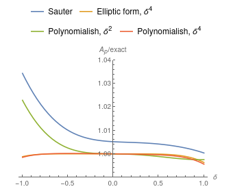
Figure 5 shows the results: our $\delta^4$ ‘Elliptic’ and ‘polynomial-ish’ approximations are much closer to the exact value. Despite having powers of $\delta^5$, at negative $\delta$ Sauter’s expression has a similar accuracy to a ‘polynomial-ish’ expression that only goes to powers of $\delta^2$.

Great! Together with the results in the previous post, we now have methods for approximating the poloidal circumference, poloidal surface area, volume, and cross-sectional area. I’ve presented the form of the derivations, and they’re generally more accurate than the approximations given by Sauter when $\delta=0$.

Written on May 31st , 2021