Particles from a Maxwellian distribution in a slab with a time-based decay probability

This problem is explored in rough analogy to the problem of ionization of neutrals coming from the wall in the edge plasma of a magnetic fusion device. This problem is almost the same as the one in the previous post, but explores a time-based interaction rather than a distance-based interaction. This allows us to consider the effect of a full velocity distribution.

Problem statement

There is a slab of material of thickness $a$. Above the slab is a gas of collisionless particles with an isotropic Maxwellian velocity distribution. When particles travel through the slab they are ionized with a mean lifetime $\tau$. Of the particles that hit the slab, what fraction will be transmitted through it? (Pretend that the velocity distribution of the particles above the slab is not affected by the absorption in the material; that would become a much more difficult problem.) Also, what is the profile of the deposition of particles within the slab?

Solving the problem

We first solve the “deposition profile” problem and then integrate to find the transmission factor.

Orient the slab normal to the (negative) z axis. In the previous problem, we needed to consider motion in the $x$ and $y$ directions, since decay was proportional to distance travelled. In this problem, the decay rate is constant with time, so to find the decay profile as a function of $z$ we only need to consider motion in $z$.

The 3D Maxwellian velocity distribution is

\[f(v_x, v_y, v_z) = \frac{1}{\left(2 \pi v_\mathrm{th}^2\right)^{3/2}} e^{-(v_x^2 + v_y^2 + v_z^2)/(2 v_\mathrm{th}^2)}\]

where $v_\mathrm{th}^2 = T/m$.

Particles with larger $v_z$ are more likely to encounter the plane. The $v_z$ distribution of these is $v_z e^{-v_z /(2 v_\mathrm{th}^2)} / v_\mathrm{th}^2$. (This is normalized so that $\int_0^\infty \; dv_z$ is 1.)
The rate of particle interaction is $\frac{1}{\tau} e^{-t/\tau}$.
Particles reach a depth $b$ after spending time $t = b/v$ in the material.
Particles spend time at a depth in the material for a time proportional to $1/v_z$.

Express this all as an integral.

Solution for deposition

The rate of particles interacting in a region of thickness $db$ around depth $b$ is

\[\begin{align} d(b, \tau v_\mathrm{th}) & = \int_0^\infty dv_z \frac{1}{\tau} e^{-b / (v_z \tau)} \frac{db}{v_z} \frac{v_z}{v_\mathrm{th}^2}e^{-v_z^2/(2 v_\mathrm{th}^2)} \\ & = \frac{db}{\tau v_\mathrm{th}^2} \int_0^\infty dv_z\; e^{-v_z^2/(2 v_\mathrm{th}^2) - b/(v_z \tau)} \\ & = \frac{db\, b}{4 \sqrt{\pi } \tau ^2 v_\mathrm{th}^2} G_{0,3}^{3,0}\left(\frac{b^2}{8 \tau^2 v_\mathrm{th}^2}\Bigg| \begin{array}{c} -\frac{1}{2},0,0 \\ \end{array} \right). \end{align}\]

(There’s no special trick here, Mathematica can just do the integral.)

Here $G$ is a Meijer G-function, a very general function with neat properties.

Solution for absorption

We can find the total absorption up to depth $a$ in the slab by integrating over $b$:

\[\mathrm{abs}(a, \tau v_\mathrm{th}) = \int_0^a \; db \frac{b}{4 \sqrt{\pi } \tau ^2 v_\mathrm{th}^2} G_{0,3}^{3,0}\left(\frac{b^2}{8 \tau^2 v_\mathrm{th}^2}\Bigg| \begin{array}{c} -\frac{1}{2},0,0 \\ \end{array} \right) = \frac{1}{\sqrt{\pi}}G_{1,4}^{3,1}\left(\frac{a^2}{8 \tau^2 v_\mathrm{th}^2 }\Bigg| \begin{array}{c} 1 \\ \frac{1}{2},1,1,0 \\ \end{array} \right).\]

It’s not surprising that this integrates well, since Meijer-G functions are closed under many operations.

The fraction of particles transmitted through the slab is $t = 1 - \mathrm{abs}$, so

\[t\left(\frac{a}{\tau v_\mathrm{th}}\right) = 1 - \frac{1}{\sqrt{\pi}}G_{1,4}^{3,1}\left(\frac{a^2}{8 \tau^2 v_\mathrm{th}^2}\Bigg| \begin{array}{c} 1 \\ \frac{1}{2},1,1,0 \\ \end{array} \right). \tag{1}\]

Alternate construction of transmission profile

We can also integrate over $b$ first, then $v_z$. The first integral is so simple it can be done in one’s head: for a slab of thickness $a$, the fraction of particles with z-velocity $v_z$ that make it through are just $e^{-a/\tau v_z}$.

Then the total transmission is

\[\begin{align} t\left(\frac{a}{\tau v_\mathrm{th}}\right) & = \int_0^\infty \frac{v_z}{v_\mathrm{th}^2}e^{-v_z^2/(2 v_\mathrm{th}^2) - a/(\tau v_z)} \; dv_z \\ & = \frac{a^2}{8 \sqrt{\pi } \tau ^2 v_\mathrm{th}^2} G_{0,3}^{3,0}\left(\frac{a^2}{8 v_\mathrm{th}^2 \tau ^2}\Bigg| \begin{array}{c} -1,-\frac{1}{2},0 \\ \end{array} \right). \\ \end{align} \tag{2}\]

Wait, what? Expressions (1) and (2) look quite different!

But, they are in fact the same thing. Meijer G-functions are very flexible.

It gets better: we can use a property that for any G-function $\mathbf{G}$, $x \mathbf{G}$ is also G-function, and get a third expression, this time all wrapped up in a single $G:$

\[t\left(\frac{a}{\tau v_\mathrm{th}}\right) = \frac{1}{\sqrt{\pi}}G_{0,3}^{3,0}\left(\frac{a^2}{8 \tau^2 v_\mathrm{th}^2 }\Bigg| \begin{array}{c} 0,\frac{1}{2},1 \\ \end{array} \right). \tag{3}\]

Nice and neat.

Mathematica code for the G-functions

x[l_, τ_, vth_] := l/(τ vth)
dep[b_, τ_, vth_]: = b MeijerG[{{}, {}}, {{-(1/2), 0, 0}, {}}, b^2/(8 vth^2 τ^2)]/(4 Sqrt[π] vth^2 τ^2)
t1[x_] := 1 - MeijerG[{{1}, {}}, {{1/2, 1, 1}, {0}}, x^2/8]/Sqrt[π]
t2[x_] := (x^2/8) MeijerG[{{}, {}}, {{-1, -(1/2), 0}, {}}, x^2/8]/Sqrt[π]
t3[x_] := MeijerG[{{}, {}}, {{0, 1/2, 1}, {}}, x^2/8]/Sqrt[π]

Characteristics of the solution

Transmission

The first figure shows the transmission curve, as well as short- and long-range asymptotics, and a standard exponential decay function for comparison. The G-function starts out looking very close to $\exp(-x)$. More precisely, the short-range asymptotic is

\[\begin{align} t(x \ll 1) & = 1 -\sqrt{\frac{\pi }{2}} x - \frac{x^2}{2}\log(x) \\ & + \frac{1}{4} x^2 \left(-2 \gamma +1+\log (8)+\psi ^{(0)}\left(-\frac{1}{2}\right)\right) \\ \end{align}\]

where $\gamma$ is Euler’s constant and $\psi^{(0)}$ is the 0th PolyGamma function. The coefficient of $x^2$ here is about 0.490 — compare to $1/2$ for a standard exponential decay, but note that the $x^2 \log(x)$ term dominates over $x^2$ for $x\ll 1$, thus I display it first.

The long-range asymptotic is $t(x \equiv a/\tau v_\mathrm{th} \gg 1 ) \sim e^{-\frac{3 x^{2/3}}{2}}\, \sqrt{2 \pi/3}\,x^{1/3} $. The $x^{2/3}$ power is pretty neat.

Deposition

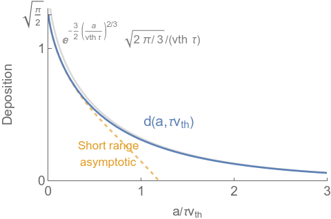
The second figure shows the profile of deposition in the slab, and the short and long-range asymptotics. Near the surface of the slab (x=0) the normalized deposition density is $\sqrt{\pi/2} \approx 1.25$ per unit, rather than 1 per unit for a standard exponential.

The 2nd-order short-range approximation is

\[d(a, \tau v_\mathrm{th}) \approx \frac{1}{\tau v_\mathrm{th}} \left(\sqrt{\frac{\pi}{2}} + \frac{x}{2} \left(\log \left(\frac{x^2}{8}\right)+2 \gamma -\psi^{(0)}\left(-\frac{1}{2}\right)\right)-\sqrt{\frac{\pi }{8}} x^2 \right)\]

where $x \equiv a/(\tau v_\mathrm{th})$.

The 1st-order long-range approximation is

\[d(a, \tau v_\mathrm{th}) \approx \frac{1}{\tau v_\mathrm{th}}\, \sqrt{2 \pi/3}\, e^{-(3/2) x^{2/3}}.\]

The G-functions are expensive to evaluate. Plotting one of these with Mathematica takes several seconds on my laptop. If you need a good-enough approximation (less than 1% error), use the 5th-order series around 0 up to x=1.5 and the 4th-order long-range asymptotic above that point.

Written on April 21st , 2024